How Are These Two Pictures Different
Last updated on July 7, 2021.
In a previous PyImageSearch blog post, I detailed how to compare two images with Python using the Structural Similarity Index (SSIM).
Using this method, we were able to easily determine if two images were identical or had differences due to slight image manipulations, compression artifacts, or purposeful tampering.
Today we are going to extend the SSIM approach so that we can visualize the differences between images using OpenCV and Python. Specifically, we'll be drawing bounding boxes around regions in the two input images that differ.
To learn more about computing and visualizing image differences with Python and OpenCV, just keep reading.
- Update July 2021: Added a section on the methods to compare images for differences and resources for additional reading about how to use siamese networks.
![]()
Looking for the source code to this post?
Jump Right To The Downloads SectionImage Difference with OpenCV and Python
In order to compute the difference between two images we'll be utilizing the Structural Similarity Index, first introduced by Wang et al. in their 2004 paper, Image Quality Assessment: From Error Visibility to Structural Similarity. This method is already implemented in the scikit-image library for image processing.
The trick is to learn how we can determine exactly where, in terms of (x, y)-coordinate location, the image differences are.
To accomplish this, we'll first need to make sure our system has Python, OpenCV, scikit-image, and imutils.
You can learn how to configure and install Python and OpenCV on your system using one of my OpenCV install tutorials.
If you don't already have scikit-image installed/upgraded, upgrade via:
$ pip install --upgrade scikit-image
While you're at it, go ahead and install/upgrade imutils as well:
$ pip install --upgrade imutils
Now that our system is ready with the prerequisites, let's continue.
Computing image difference
Can you spot the difference between these two images?

If you take a second to study the two credit cards, you'll notice that the MasterCard logo is present on the left image but has been Photoshopped out from the right image.
You may have noticed this difference immediately, or it may have taken you a few seconds. Either way, this demonstrates an important aspect of comparing image differences — sometimes image differences are subtle — so subtle that the naked eye struggles to immediately comprehend the difference (we'll see an example of such an image later in this blog post).
So why is computing image differences so important?
One example is phishing. Attackers can manipulate images ever-so-slightly to trick unsuspecting users who don't validate the URL into thinking they are logging into their banking website — only to later find out that it was a scam.
Comparing logos and known User Interface (UI) elements on a webpage to an existing dataset could help reduce phishing attacks (a big thanks to Chris Cleveland for passing along PhishZoo: Detecting Phishing Websites By Looking at Them as an example of applying computer vision to prevent phishing).
Developing a phishing detection system is obviously much more complicated than simple image differences, but we can still apply these techniques to determine if a given image has been manipulated.
Now, let's compute the difference between two images, and view the differences side by side using OpenCV, scikit-image, and Python.
Open up a new file and name it image_diff.py , and insert the following code:
# import the necessary packages from skimage.metrics import structural_similarity as compare_ssim import argparse import imutils import cv2 # construct the argument parse and parse the arguments ap = argparse.ArgumentParser() ap.add_argument("-f", "--first", required=True, help="first input image") ap.add_argument("-s", "--second", required=True, help="second") args = vars(ap.parse_args()) Lines 2-5 show our imports. We'll be using compare_ssim (from scikit-image), argparse , imutils , and cv2 (OpenCV).
We establish two command line arguments, --first and --second , which are the paths to the two respective input images we wish to compare (Lines 8-13).
Next we'll load each image from disk and convert them to grayscale:
# load the two input images imageA = cv2.imread(args["first"]) imageB = cv2.imread(args["second"]) # convert the images to grayscale grayA = cv2.cvtColor(imageA, cv2.COLOR_BGR2GRAY) grayB = cv2.cvtColor(imageB, cv2.COLOR_BGR2GRAY)
We load our first and second images, --first and --second , on Lines 16 and 17, storing them as imageA and imageB , respectively.
Then we convert each to grayscale on Lines 20 and 21.

Next, let's compute the Structural Similarity Index (SSIM) between our two grayscale images.
# compute the Structural Similarity Index (SSIM) between the two # images, ensuring that the difference image is returned (score, diff) = compare_ssim(grayA, grayB, full=True) diff = (diff * 255).astype("uint8") print("SSIM: {}".format(score)) Using the compare_ssim function from scikit-image, we calculate a score and difference image, diff (Line 25).
The score represents the structural similarity index between the two input images. This value can fall into the range [-1, 1] with a value of one being a "perfect match".
The diff image contains the actual image differences between the two input images that we wish to visualize. The difference image is currently represented as a floating point data type in the range [0, 1] so we first convert the array to 8-bit unsigned integers in the range [0, 255] (Line 26) before we can further process it using OpenCV.
Now, let's find the contours so that we can place rectangles around the regions identified as "different":
# threshold the difference image, followed by finding contours to # obtain the regions of the two input images that differ thresh = cv2.threshold(diff, 0, 255, cv2.THRESH_BINARY_INV | cv2.THRESH_OTSU)[1] cnts = cv2.findContours(thresh.copy(), cv2.RETR_EXTERNAL, cv2.CHAIN_APPROX_SIMPLE) cnts = imutils.grab_contours(cnts)
On Lines 31 and 32 we threshold our diff image using both cv2.THRESH_BINARY_INV and cv2.THRESH_OTSU — both of these settings are applied at the same time using the vertical bar 'or' symbol, | . For details on Otsu's bimodal thresholding setting, see this OpenCV documentation.
Subsequently we find the contours of thresh on Lines 33-35. The ternary operator on Line 35 simply accommodates difference between the cv2.findContours return signature in various versions of OpenCV.
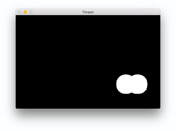
The image in Figure 4 below clearly reveals the ROIs of the image that have been manipulated:
Now that we have the contours stored in a list, let's draw rectangles around the different regions on each image:
# loop over the contours for c in cnts: # compute the bounding box of the contour and then draw the # bounding box on both input images to represent where the two # images differ (x, y, w, h) = cv2.boundingRect(c) cv2.rectangle(imageA, (x, y), (x + w, y + h), (0, 0, 255), 2) cv2.rectangle(imageB, (x, y), (x + w, y + h), (0, 0, 255), 2) # show the output images cv2.imshow("Original", imageA) cv2.imshow("Modified", imageB) cv2.imshow("Diff", diff) cv2.imshow("Thresh", thresh) cv2.waitKey(0) Beginning on Line 38, we loop over our contours, cnts . First, we compute the bounding box around the contour using the cv2.boundingRect function. We store relevant (x, y )-coordinates as x and y as well as the width/height of the rectangle as w and h .
Then we use the values to draw a red rectangle on each image with cv2.rectangle (Lines 43 and 44).
Finally, we show the comparison images with boxes around differences, the difference image, and the thresholded image (Lines 47-50).
We make a call to cv2.waitKey on Line 50 which makes the program wait until a key is pressed (at which point the script will exit).

Next, let's run the script and visualize a few more image differences.
Visualizing image differences
Using this script and the following command, we can quickly and easily highlight differences between two images:
$ python image_diff.py --first images/original_02.png --second images/modified_02.png
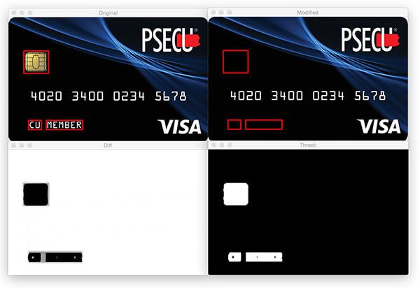
As you can see in Figure 6, the security chip and name of the account holder have both been removed:
Let's try another example of computing image differences, this time of a check written by President Gerald R. Ford (source).
By running the command below and supplying the relevant images, we can see that the differences here are more subtle:
$ python image_diff.py --first images/original_03.png --second images/modified_03.png
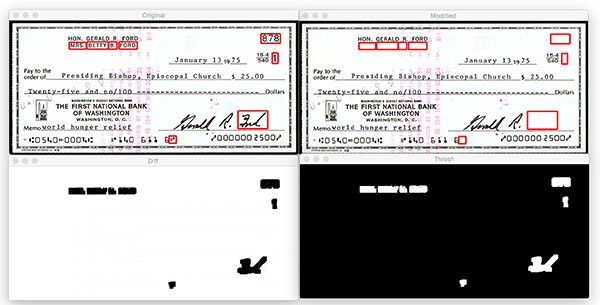
Notice the following changes in Figure 7:
- Betty Ford's name is removed.
- The check number is removed.
- The symbol next to the date is removed.
- The last name is removed.
On a complex image like a check it is often difficult to find all the differences with the naked eye. Luckily for us, we can now easily compute the differences and visualize the results with this handy script made with Python, OpenCV, and scikit-image.
Other methods to compare images for differences
This tutorial covered how to use the Structural Similarity Index (SSIM) to compare two images and spot differences between the two.
SSIM is a traditional computer vision approach to image comparison; however, there are other image difference algorithms that can be utilized, specifically deep learning ones.
To start, one could apply transfer learning by:
- Selecting a pre-trained CNN (ResNet, VGGNet, etc.) on a large, diverse image dataset (e.g., ImageNet)
- Removing the fully connected layer head from the network
- Passing all images in your dataset through the CNN and extracting the features from the final layer
- Computing a k-Nearest Neighbor comparison between the features and then finding the most similar images to the input query
However, keep in mind that the k-NN approach does not actually "learn" any underlying patterns/similarity scores in images in your dataset.
To actually learn image differences and make robust comparisons between them, you should utilize siamese networks.
The following tutorials will teach you about siamese networks:
- Building image pairs for siamese networks with Python
- Siamese networks with Keras, TensorFlow, and Deep Learning
- Comparing images for similarity using siamese networks, Keras, and TensorFlow
- Contrastive Loss for Siamese Networks with Keras and TensorFlow
Additionally, siamese networks are covered in detail inside PyImageSearch University.
What's next? I recommend PyImageSearch University.
Course information:
28 total classes • 39h 44m video • Last updated: 10/2021
★★★★★ 4.84 (128 Ratings) • 3,000+ Students Enrolled
I strongly believe that if you had the right teacher you could master computer vision and deep learning.
Do you think learning computer vision and deep learning has to be time-consuming, overwhelming, and complicated? Or has to involve complex mathematics and equations? Or requires a degree in computer science?
That's not the case.
All you need to master computer vision and deep learning is for someone to explain things to you in simple, intuitive terms. And that's exactly what I do. My mission is to change education and how complex Artificial Intelligence topics are taught.
If you're serious about learning computer vision, your next stop should be PyImageSearch University, the most comprehensive computer vision, deep learning, and OpenCV course online today. Here you'll learn how to successfully and confidently apply computer vision to your work, research, and projects. Join me in computer vision mastery.
Inside PyImageSearch University you'll find:
- ✓ 28 courses on essential computer vision, deep learning, and OpenCV topics
- ✓ 28 Certificates of Completion
- ✓ 39h 44m on-demand video
- ✓ Brand new courses released every month , ensuring you can keep up with state-of-the-art techniques
- ✓ Pre-configured Jupyter Notebooks in Google Colab
- ✓ Run all code examples in your web browser — works on Windows, macOS, and Linux (no dev environment configuration required!)
- ✓ Access to centralized code repos for all 400+ tutorials on PyImageSearch
- ✓ Easy one-click downloads for code, datasets, pre-trained models, etc.
- ✓ Access on mobile, laptop, desktop, etc.
Click here to join PyImageSearch University
Summary
In today's blog post, we learned how to compute image differences using OpenCV, Python, and scikit-image's Structural Similarity Index (SSIM). Based on the image difference we also learned how to mark and visualize the different regions in two images.
To learn more about SSIM, be sure to refer to this post and the scikit-image documentation.
I hope you enjoyed today's blog post!
And before you go, be sure to enter your email address in the form below to be notified when future PyImageSearch blog posts are published!

Download the Source Code and FREE 17-page Resource Guide
Enter your email address below to get a .zip of the code and a FREE 17-page Resource Guide on Computer Vision, OpenCV, and Deep Learning. Inside you'll find my hand-picked tutorials, books, courses, and libraries to help you master CV and DL!
How Are These Two Pictures Different
Source: https://www.pyimagesearch.com/2017/06/19/image-difference-with-opencv-and-python/